Kinetic Analysis
Starting in Labrador v2.2.0, some metrics will be calculated for growth curves automatically. These values are calculated by fitting normalized data to this version of the Richard’s growth model. When the minimum datum is below 0, then the following formula is applied to normalize the data above 0 normalized data set = data - minimum of dataset. This normalization is crucial because, in subsequent calculations, the logarithm of the dataset is utilized. It’s important to note that this logarithmic operation requires non-negative data to prevent undefined values from polluting calculations. The graph displayed in the Analysis tab shows the normalized data, so it may have slightly higher y values than the data presented in Plate Results and Graph Results. Metrics in the table are grouped by metrics that are calculated from the raw data without using the fitted model at all and data that is calculated from the chosen growth model fit to the data.
Number |
Element |
Description |
|---|---|---|
1 |
Metrics Table – Copy |
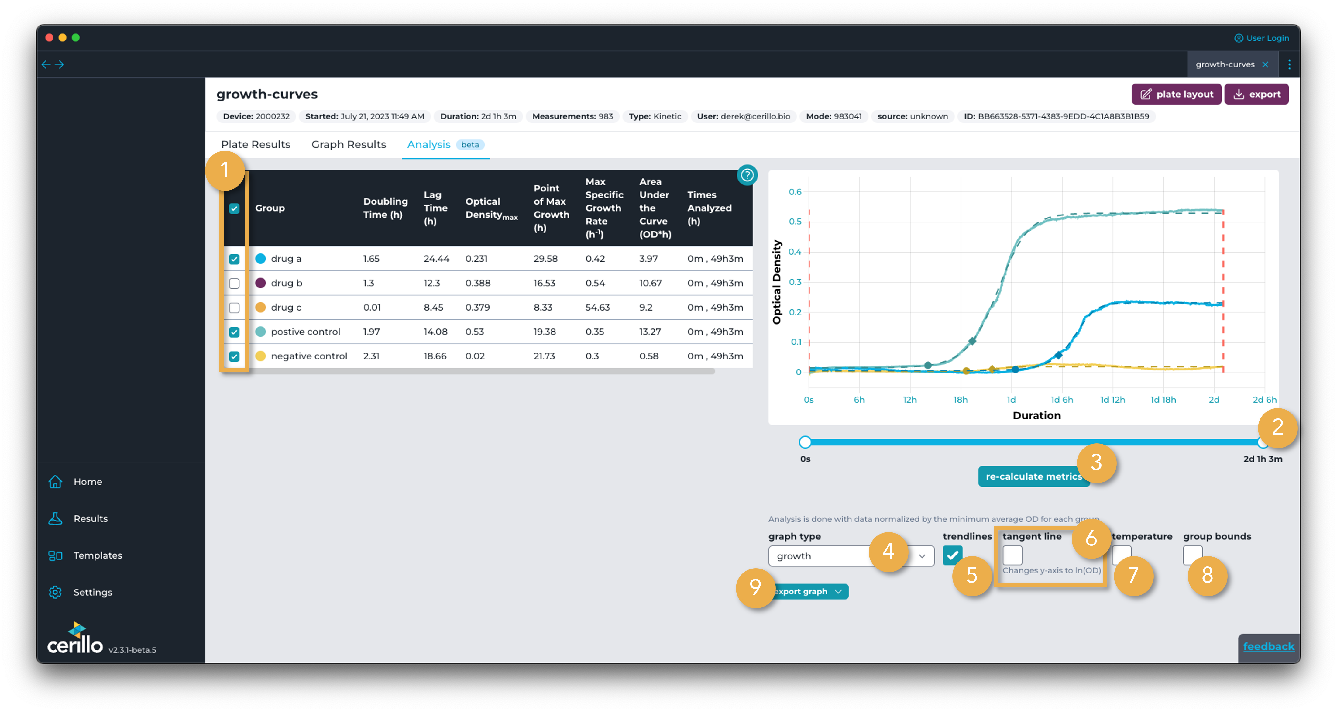
Click to copy the metrics table into the clipboard for pasting into a spreadsheet program. |
2 |
Metrics Table – Group toggle |
Click the header checkbox to toggle visibility on and off for all groups. Click a group checkbox to toggle visibility on or off for that specific group. Group visibility also controls what groups will be affected by bounding changes made with the re-calculate metrics button. Clicking the header of other metrics will sort the table and graph to that metric. |
3 |
Export Graph |
Export the graph as a |
4 |
More information |
Open up user manual for analysis tools. |
5 |
Bound Slider |
Slider that controls the start and end times of the data fed to the model when re-calculate metrics is clicked. See bounding-model for more details. |
6 |
Analysis Function Select |
Choose between available growth models used to fit the data and calculate metrics. |
7 |
Re-calculate Metrics |
Click update the start and end times of data fed to the models for every group currently visible to the red dotted vertical lines. |
8 |
Graph Type Select |
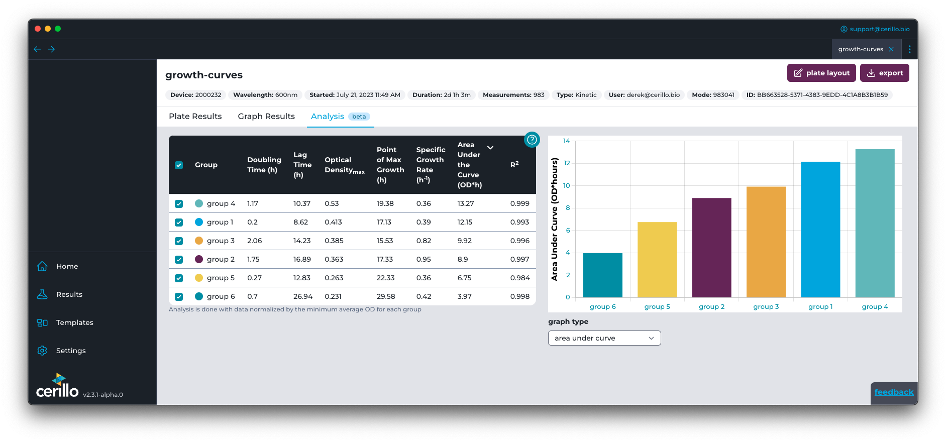
Choose between growth, which is the typical kinetic graph results view, to bar charts comparing each metric in the table on the right. See metric comparison for an example. |
9 |
Group Bounds |
Toggle the group bounds used to calculate metrics for each individual group. Note that these will be the extents of the graph unless a change to the Bound Slider is changed and Re-calculate Metrics is clicked |
10 |
Trend Lines |
Toggle on the model for each group as a dotted line. Will also display lag time estimate and point of max specific growth as a circle and diamond, respectively |
11 |
Temperature |
Toggle on temperature data in the growth chart |
12 |
Tangent Lines |
Updates growth chart to logarithmic y-axis. Toggles on visibility of tangent lines at the point of max specific growth. The slope of the tangent line is equal to 𝜇𝑚𝑎𝑥. |
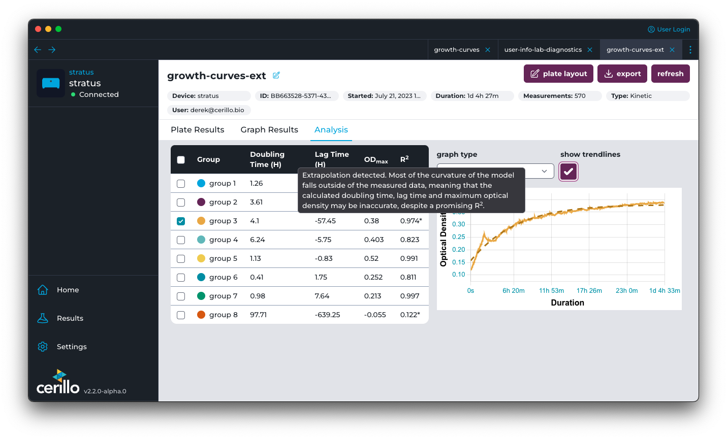
Certain rows may be highlighted if the fit of the growth model should not be trusted, either because of a low R2 value, or because extrapolation was detected. When this is the case, one should take caution in using any of the metrics calculated from the model fit. Metrics calculated directly from raw data values are still valid for these rows.
Symbol |
Color |
Description |
|---|---|---|
⚠️ |
Red |
Low R2 <0.8 detected in model fit. |
* |
Orange |
Extrapolation detected in model fit. |
Tip
At least one group with wells assigned to it must be present in the plate layout for Labrador to analyze growth data
Growth Model
Multiple growth models are available to calculate lag time, doubling time and specific growth rate. Those models include:
Richards Model
Gompertz Model
Richards Model
The growth model used within Labrador is a modified Richards Curve with the following form:

Parameter |
Description |
|---|---|
A > 0 |
The lower (left) asymptote. Minimum value of 0. This helps keep the maximum specific growth rate reasonable, as a negative A will produce a vertical asymptote in the logarithmic space. |
K |
The upper (right) asymptote. Carrying capacity. Optical Densitymax |
r > 0 |
The intrinsic growth rate. Minimum value of 0, meaning that decay data – rather than growth data – will not yield accurate metrics. |
𝛾 |
The inflection point where logarithmic growth ends. |
t |
The time elapsed |
𝜈 > 0 |
Asymmetry parameter - describes the transition between growth phases. |
f(t) |
Optical Density |
Gompertz Model

Parameter |
Description |
|---|---|
A > 0 |
The lower (left) asymptote. Minimum value of 0. This helps keep the maximum specific growth rate reasonable, as a negative A will produce a vertical asymptote in the logarithmic space. |
K |
The upper (right) asymptote. Carrying capacity. Optical Densitymax |
μm |
Max specific growth rate |
t |
The time elapsed |
λ |
Lag time before exponential growth. |
f(t) |
Optical Density |
Calculating metrics from the model
From the growth model, the lag time, doubling time, and maximum optical density can be derived, which are displayed in the analysis tab of kinetic results.
The max specific growth rate (𝜇𝑚𝑎𝑥) is calculated by finding the max derivative of the natural logarithm of the model equation. We use the model equation instead of the raw data to avoid noise. See Logarithmic Visualization for how to visualize 𝜇𝑚𝑎𝑥.

Doubling time (Td) is derived from the specific max growth rate with the following equation, which is true under constant continuous growth rate r:

The lag time is calculated by finding the intersection of left asymptote A (the initial population size) with the max specific growth rate tangent line in logarithmic coordinates. If A is negative, then the initial optical density is used instead. For the Gompertz model, the lag time is one of the parameters of the equation, so it does not need to be calculated post-fitting.
Area under the curve is calculated with a trapezoid approximation of the integral of the measured data. It does not make use of the growth model fit.
Logarithmic Visualization
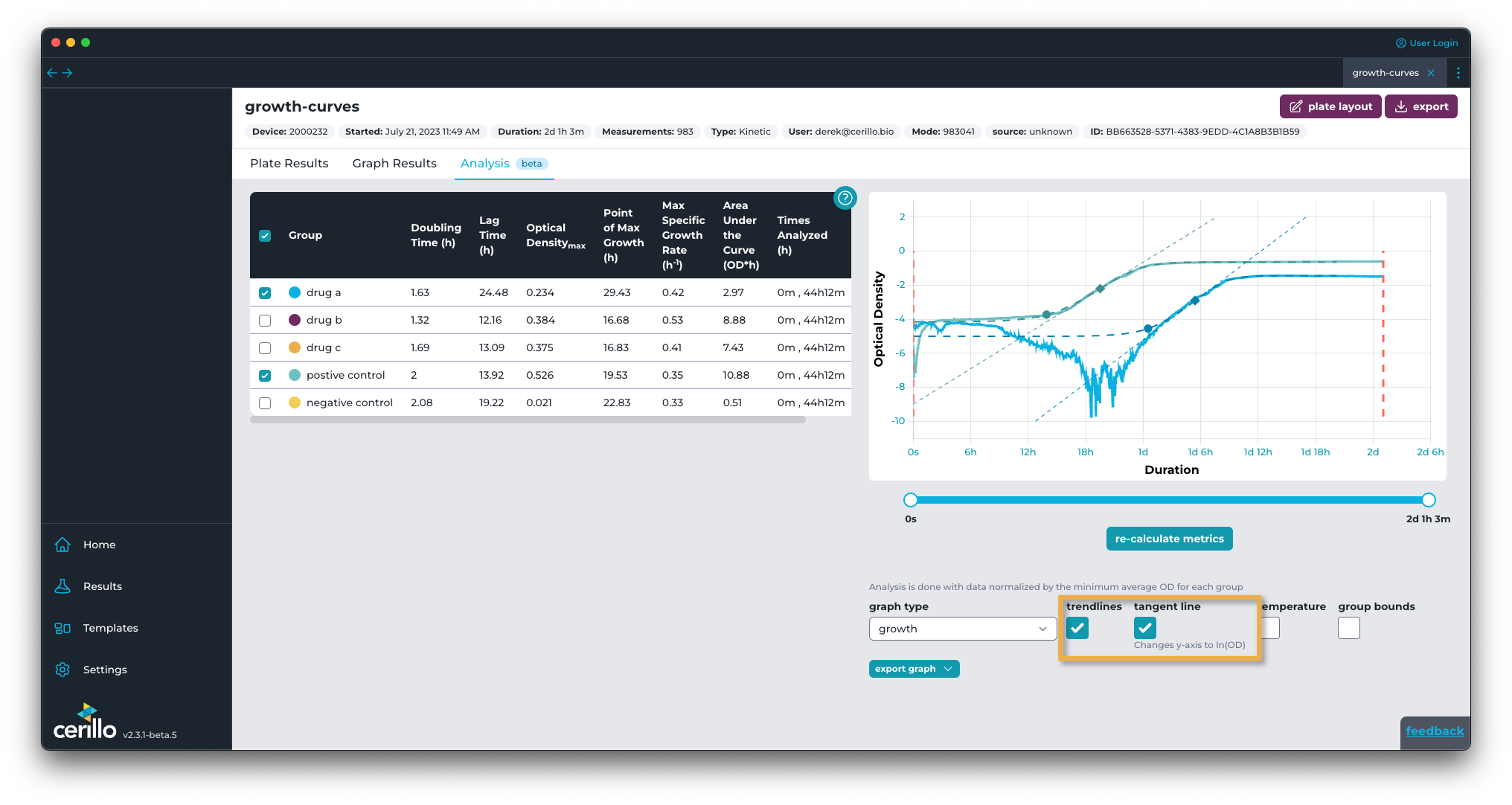 Since 𝜇𝑚𝑎𝑥, doubling time, and lag time are derived from the natural logarithm of the OD, it can be useful to visualize the data with ln(OD). Toggling on the tangent line at 𝜇𝑚𝑎𝑥 will convert the graph to ln(OD).
Note
Since a negative OD value will result in a logarithm of -infinity, we normalize the data to be above 0 and enforce the model to make the lower-asymptote > 0. If the logarithmic graph approaches is -infinity to the left, then the 𝜇𝑚𝑎𝑥 will be erroneously very large and the doubling time very low.
Bounding Model
In some circumstances, it may be useful to bound the kinetic model’s start and end time to improve accuracy of metrics. For instance, if inoculation occurs mid-experiment, you may want to fit the kinetic model after inoculation has occurred. Or, you may want to filter out the death phase of bacteria to improve the R2 of the fit. This can be accomplished within Labrador on a per-group basis.
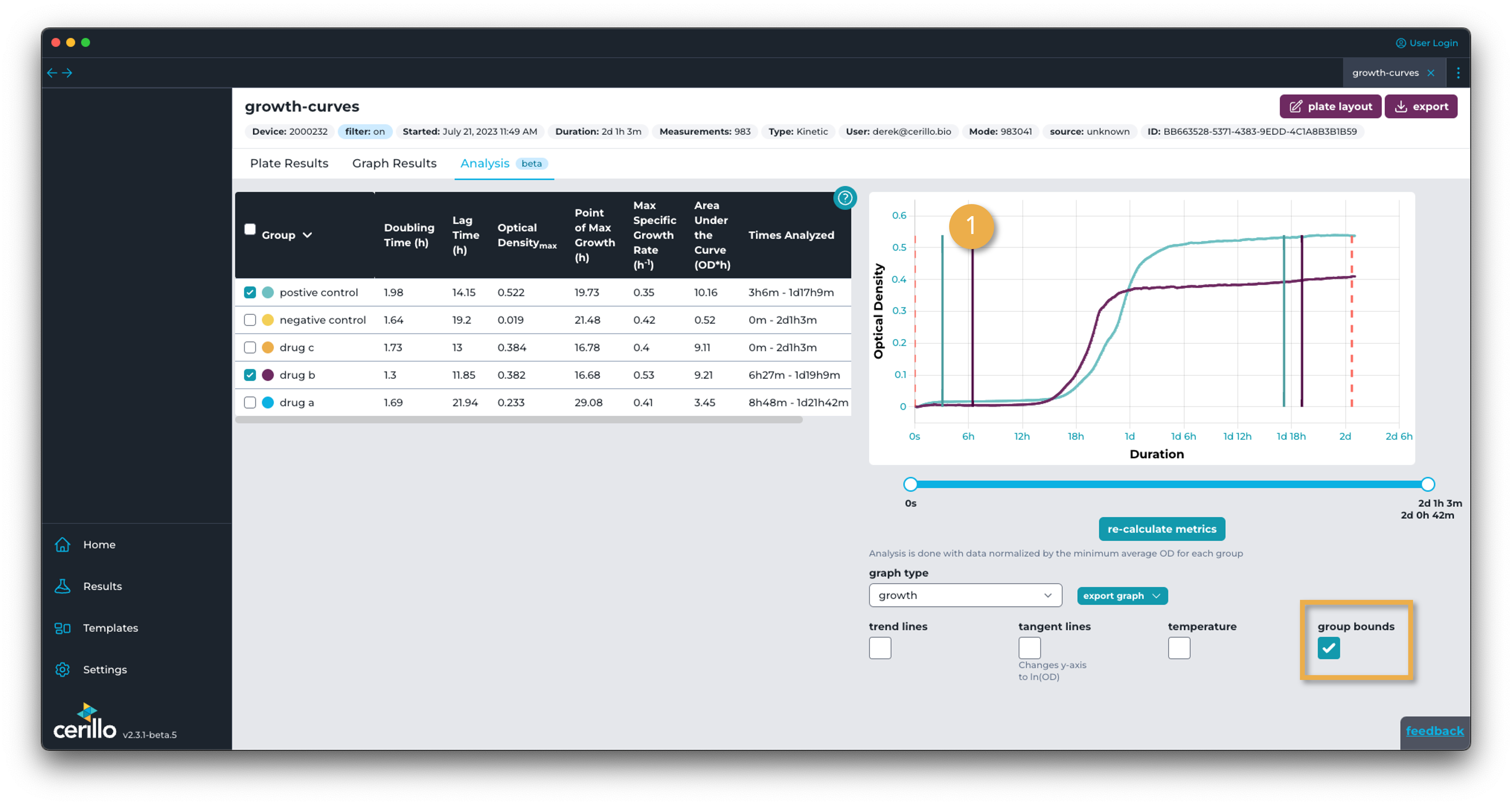
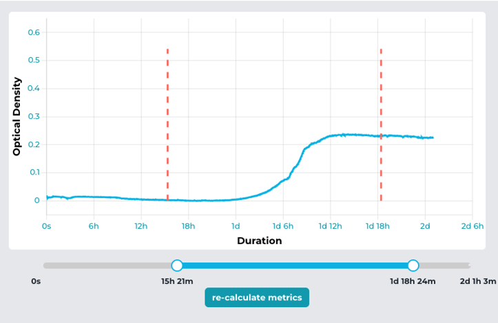 Use the slider to edit the start and end time of data fed to the model to be fit. The left-most handle controls the start time while the right-most handle controls the end time. The dotted vertical red lines in the graph view display the pending start and end times. Upon clicking re-calculate metrics the start and end times for ALL visible groups will be updated to the pending start and end times. The red dotted bounds only mark pending changes to model bounds. To view the current values for each visible group, use the group bounds toggle. The start and end times for each group will display as solid vertical lines of the same color as the group, as seen in number 1 below:
Extrapolation detection
In some cases where data is linear or the experiment is started near saturation, the model can be highly-extrapolated which means that the metrics should not necessarily be trusted. When extrapolation is detected, an asterisk will appear next to the R2 value.
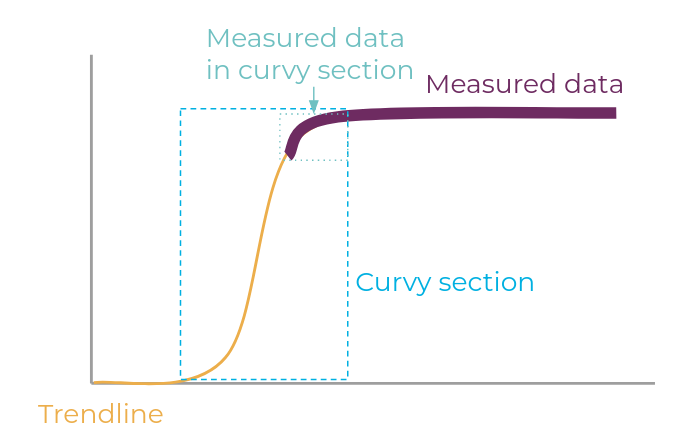
Extrapolation detection works by analyzing the curvy section of the model and comparing that to the curvy section of the measured data. If the width of the measured curvy section is less than half of the curvy section of the model overall, the data will be marked as extrapolated.
Metric Comparison